
Plotting integrated data
I recently created a graph that shows how much CPU time a number of processes
took before they terminated.
For this, I ran my processes with the time command, such as:
/usr/bin/time -o command.time <command>
This produces a file “command.time” like the following:
7.91user 0.08system 0:08.00elapsed 99%CPU (0avgtext+0avgdata 168352maxresident)k
0inputs+8outputs (0major+21257minor)pagefaults 0swaps
When we have several of such files, we might be interested in showing at which points in time every command terminated. For this, let us assume we have a directory with several “.time” files. Let us first filter out the unnecessary lines:
cat *.time | grep "elapsed"
That gives something like:
3.22user 0.23system 0:03.47elapsed 99%CPU (0avgtext+0avgdata 908592maxresident)k
3.93user 0.44system 0:04.41elapsed 99%CPU (0avgtext+0avgdata 722864maxresident)k
0.87user 0.04system 0:00.92elapsed 99%CPU (0avgtext+0avgdata 86576maxresident)k
0.39user 0.06system 0:00.46elapsed 99%CPU (0avgtext+0avgdata 89088maxresident)k
[...]
For the sake of this example, we are only interested in the user time,
which roughly corresponds to the time the program was working itself,
in contrast to the time it waited for the kernel to perform tasks.
So let us cut away every but the first column:
cat *.time | grep "elapsed" | cut -d "u" -f 1
(The “-d” option specifies a delimiter, and the “-f” option specifies that only the first field before a delimiter should be output.)
The output of this is:
3.22
3.93
0.87
0.39
[...]
Now I want a graph that makes a tiny “jump” at every point in time given by the data above, thus integrating over all the data. For this task, I created a Haskell program “integrate.hs”:
import Control.Category ((>>>))
import Data.List (sort)

process =
  lines >>>
  map read >>>
  sort >>>
  scanl (\ (_, y) x -> (x, y+1)) (0 :: Double, 0) >>>
  map (\ (x, y) -> show x ++ " " ++ show y)

main = getContents >>= return . process >>= mapM putStrLn
Compile it with ghc integrate.hs, yielding an executable “integrate”.
(EDIT 2021-03-01: Instead of using Haskell here,
a slightly more low-tech solution is to just pipe through
sort -n | awk '{print $0 " " NR}'.
In the awk script,
$0 refers to the current line, and
NR refers to the current line number.)
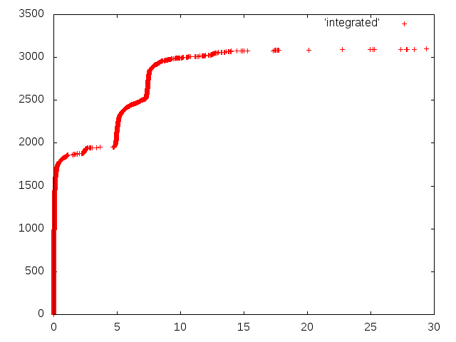
Now you can use gnuplot to see the final result:
cat *.time | grep "elapsed" | cut -d "u" -f 1 | ./integrate > integrated
gnuplot -e "plot 'integrated'; pause -1"
To plot it to a PNG file:
gnuplot -e "set term png; set output 'gnuplot.png'; plot 'integrated'"
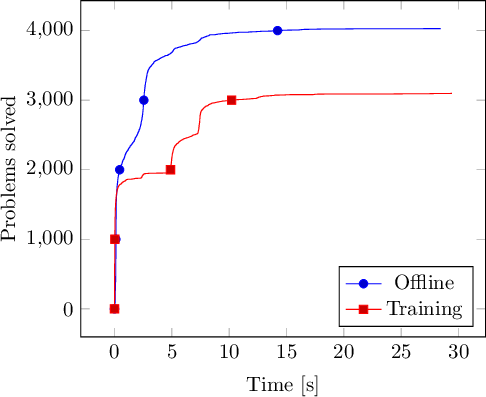
If you want to display the resulting plot in LaTeX, you can use TikZ:
\documentclass[preview]{standalone}

\usepackage{pgfplots}
\pgfplotsset{compat=1.9}
\usepgfplotslibrary{units}

\begin{document}

\begin{tikzpicture}
\begin{axis}
[ legend pos=south east
, xlabel=Time
, x unit=s
, ylabel=Problems solved
, mark repeat={1000}
]
\addplot table {offline.integrated};
\addlegendentry{Offline};
\addplot table {training.integrated};
\addlegendentry{Training};
\end{axis}
\end{tikzpicture}

\end{document}
To compile it:
pdflatex tikz.tex
convert -density 150 tikz.pdf -quality 90 -trim tikz.png
Voilà ! Have fun creating your own integrated data plots!